- Published on
- |Views: 0|63 min read| Draft
Outperforming Native PyTorch Ops on Apple Silicon with Custom Metal Kernels
- Authors

- Name
- Shashank Shekhar
- @sshkhr16
All code from this post is available in this GitHub repository: github.com/sshkhr/metal-layernorm-torch
In this post, we will iteratively optimize a LayerNorm kernel written in Metal and integrated into PyTorch's MPS backend. My goal with this project is to deeply understand (and explain) how to write, profile, and optimize GPU compute kernels on Apple Silicon, because the existing resources for doing this are somewhat thin.
The CUDA ecosystem has Nsight Compute, a decade of community wisdom, and several fantastic blog posts like Simon Boehm's matmul worklog that walk through kernel optimization from first principles. Metal has Xcode's GPU trace, a handful of WWDC talks from Apple, and tutorials that pretty much stop at "hello world" matrix multiplication. For a deeper dive, the only option is to read source code from the PyTorch MPS backend or the MLX package. This post tries to be the resource I wished existed when I started.
I chose LayerNorm specifically because it is a memory(bandwidth)-bound operation and does very little arithmetic relative to the data it moves. That makes it a great lens for studying Apple Silicon's memory hierarchy, which is architecturally quite different from NVIDIA GPUs. These differences mean CUDA optimization intuitions don't always transfer, and the sometimes only way to learn what does and doesn't work is by trying.
We'll start with a naive kernel that achieves ~5 GB/s and progressively optimize it until we can surpass PyTorch's native LayerNorm on my M1 Max GPU. Each kernel is motivated by a specific bottleneck visible in the previous kernel's GPU profile, so the post doubles as a tutorial on Metal's profiling tools (introduced one at a time as the optimization demands them). I should note that I'm not a Metal expert; I came to this from the CUDA side and learned by doing. Corrections and suggestions are very welcome!
This post tries its best to be self-contained, and explains GPU hardware and software concepts as we encounter them. If you'd like, you can build some familiarity with the basic concepts (threads, threadgroups/blocks, global memory, shared memory, etc) by reading the CUDA Refresher. If you need a mapping from CUDA to Metal terminology, I've written a detailed comparison in Apple Silicon Metal vs NVIDIA CUDA, covering the architecture, memory hierarchy, and programming model side by side.
Setting Up Custom Metal Kernels in PyTorch
Before we run or profile our Metal kernels, we need to integrate them with PyTorch. Metal is its own DSL (domain specific language) for writing Apple Silicon GPU code, and unlike some other DSLs (like Triton) doesn't come with a Python API that can directly plug into PyTorch. There are two ways to do integrate Metal into PyTorch:
Approach 1: Just-in-Time Compilation with load_inline()
torch.utils.cpp_extension.load_inline lets us load custom C++ based extensions directly into Pytorch. From the Pytorch docs:
load_inline() takes its sources as strings which are stored to files in the build directory. A Ninja build file is emitted, which is used to compile the given sources into a dynamic library. This library is subsequently loaded into the current Python process as a module and returned from this function, ready for use.This is the approach used in Gimlet Labs' AI-generated metal kernels post. It's the fastest path for prototyping, but load_inline() pulls in all of libtorch's headers, resulting in longer compilation times for kernels. This is fine for a one-off experiments, but it wastes too much time during iterative development and benchmarking several runs.
Approach 2: Ahead-of-Time Compilation with setuptools
We can build a proper installable Python package that compiles the Objective-C++ dispatch code once with a standard setup.py workflow and ships .metal shader files as package data. This is the approach we use, and the approach PyTorch's own MPS backend uses internally. This approach allows for faster iteration (rebuild only what changed), clean separation of Metal shaders from dispatch logic, and a standard pip install -e . workflow.
For this project, we use the pre-compiled approach. The diagram below shows how all the pieces fit together. I borrowed this setup from the pytorch-cpp-metal-tutorial repo and Custom PyTorch Operations for Metal Backend blog post, which are both good starting points if you want to understand how to pre-compile custom Metal kernels into Pytorch C++ extensions. But I will do a deeper dive into the setup here for completeness.

Let's walk through each part of this architecture in detail, starting with the build system and dispatch layer.
The Build System
Metal primarly provides a Swift and Objective-C API for GPU programming. There's also a C++ only API (metal-cpp), but since PyTorch's CppExtension can build Objective-C++ files (a mixture of Objective-C and C++ code), we will just use the Objective-C++ API. However, it requires a small patch since setuptools doesn't recognize .mm files by default:
from distutils.unixccompiler import UnixCCompiler
if '.mm' not in UnixCCompiler.src_extensions:
    UnixCCompiler.src_extensions.append('.mm')
    UnixCCompiler.language_map['.mm'] = 'objc'
Without this, the build silently skips our dispatch code and produces a broken extension with zero Metal functionality. The rest of setup.py links against the Metal and Foundation frameworks and ships the .metal files as package data:
ext = CppExtension(
    name='layernorm_metal._C',
    sources=['src/dispatch.mm'],
    extra_compile_args={'cxx': ['-std=c++17', '-ObjC++', '-Wall']},
    extra_link_args=['-framework', 'Metal', '-framework', 'Foundation'],
)
The -ObjC++ flag forces Clang to treat the source as Objective-C++, required for @autoreleasepool, [object method:] syntax, and Metal framework types. The .metal shader files are not compiled at build time — they ship as source and get compiled to GPU instructions at runtime via newLibraryWithSource:.
We can now install this like a regular Python package with pip install -e . and we're ready to dispatch Metal compute from Python.
The Python Wrapper
The wrapper layer (wrapper.py) maps human-readable kernel names to .metal file paths and forwards calls to the compiled C++ extension:
KERNELS = {
    "naive":      ("layernorm_naive.metal",      "layernorm_naive"),
    "shared":     ("layernorm_shared.metal",     "layernorm_shared"),
    "simd":       ("layernorm_simd.metal",       "layernorm_simd"),
    "vectorized": ("layernorm_vectorized.metal", "layernorm_vectorized"),
    # ... and other kernels
}

def layernorm_forward(input, gamma, beta, eps=1e-5, kernel="vectorized"):
    filename, kernel_name = KERNELS[kernel]
    return _C.layernorm_forward(
        input, gamma, beta, eps, _shader_path(filename), kernel_name
    )
This lets user code stay clean — layernorm_forward(x, gamma, beta, kernel="simd") — while the wrapper handles file path resolution via pkg_resources.
The Dispatch Layer: What's Different from Standard Metal
The Objective-C++ dispatch code in dispatch.mm follows the standard Metal dispatch pipeline: device → library → function → pipeline state → command buffer → encoder → dispatch → commit. If you're unfamiliar with this pipeline, I cover it in detail alongside the equivalent CUDA code in Apple Silicon Metal vs NVIDIA CUDA.
The PyTorch integration follows the same pipeline with three key adaptations that we won't find in the standard Metal tutorials:
1. Borrowing PyTorch's command buffer
MTLCommandBuffer.Standard Metal code creates its own command queue and command buffers. In the PyTorch integration, we borrow PyTorch's internal command buffer so that our kernel executes in the correct order relative to PyTorch's own MPS operations:
id<MTLCommandBuffer> cmdBuf = torch::mps::get_command_buffer();
dispatch_queue_t queue = torch::mps::get_dispatch_queue();

dispatch_sync(queue, ^(){
    id<MTLComputeCommandEncoder> enc = [cmdBuf computeCommandEncoder];
    // ... encode kernel ...
    [enc endEncoding];
    torch::mps::commit();
});
get_command_buffer() returns the current command buffer that PyTorch uses for all MPS ops — our kernel's work is encoded into the same buffer, ensuring correct GPU execution ordering. get_dispatch_queue() returns a serial queue that serializes all Metal command encoding, preventing race conditions when multiple threads try to encode simultaneously. commit() submits the command buffer to the GPU. All three calls must happen inside the dispatch_sync block.
2. Extracting Metal buffers from PyTorch tensors
MTLBuffer is Metal's GPU-accessible memory allocation — the equivalent of a CUDA device pointer, but wrapped as an Objective-C object with size and storage mode metadata.Standard Metal code allocates its own MTLBuffer objects. PyTorch MPS tensors are already backed by Metal buffers — we just need to extract the handle:
static inline id<MTLBuffer> getMTLBufferStorage(const torch::Tensor& tensor) {
    return __builtin_bit_cast(id<MTLBuffer>, tensor.storage().data());
}
For MPS tensors, tensor.storage().data() returns a void* that is actually the raw pointer representation of an Objective-C id<MTLBuffer> object. __builtin_bit_cast (C++20's std::bit_cast) performs a zero-cost bit-level reinterpretation without triggering Automatic Reference Counting interference — using reinterpret_cast here would cause ARC to try to manage the Objective-C object's lifetime, leading to crashes. When setting buffer offsets on the encoder, we account for tensor views via tensor.storage_offset() * tensor.element_size().
3. Pipeline state caching
MTLComputePipelineState) is Metal's compiled, GPU-ready representation of a shader function — analogous to a compiled CUDA module (cuFunction).Standard Metal tutorials create the pipeline state inline. When benchmarking kernels over thousands of iterations, this becomes a critical performance bug:
// ❌ Without caching: compiles the shader on EVERY call
id<MTLDevice> device = MTLCreateSystemDefaultDevice();
id<MTLLibrary> lib = [device newLibraryWithSource:src options:nil error:&error];
id<MTLComputePipelineState> pso = [device newComputePipelineStateWithFunction:fn error:&error];
Metal shader compilation takes milliseconds. If our kernel runs in microseconds, compiling the shader on every invocation creates massive pipeline bubbles — the GPU finishes a kernel, then sits idle while the CPU compiles the next shader. GPU caches go completely cold between iterations. Our PipelineCache compiles each (shader_path, kernel_name) pair exactly once and returns cached pipeline states on subsequent calls. In our benchmarks, this single fix produced a 10× improvement in measured throughput at small batch sizes.
LayerNorm: Napkin Math
For this project, we will be implementing and optimizing LayerNorm, an operator quite commonly used in transformer-based as well as other deep learning architectures. There are already reference examples for CUDA: Arya's blog post on optimizing LayerNorm is a great intro to CUDA optimization, with excellent illustrations for visual learners. OneFlow team's blog post is a more in-depth guide that covers Welford's algorithm and optimizations across batch sizes.
We will see shortly why LayerNorm is also an excellent case study for the unique memory hierarchy and SIMD capabilities of Apple Silicon. We will be developing the toolkit for profiling and optimizing GPU kernels on Apple Silicon along the way, which is a transferable skill to any operator we might want to implement.
LayerNorm computes, per row of an input matrix:
where and , with learnable scale and bias .
Before writing any code, let's work through the arithmetic to understand what kind of kernel we're writing. Per element, LayerNorm requires approximately 8 FLOPs:
- 1 add for mean accumulation
- 3 ops for variance (subtract, multiply, add)
- 2 ops for normalization (subtract, multiply by rsqrt)
- 2 ops for the affine transform (multiply by , add )
Bandwidth Is All You Need
Now let's count the bytes moved for the LayerNorm operation. How many bytes we move depends on how many passes the kernel makes over the input:
| Algorithm | Passes over | Bytes per element | Description |
|---|---|---|---|
| 3-pass | 3 reads + 1 write | B | Mean, variance, normalize as separate loops |
| 2-pass | 2 reads + 1 write | B | Fuse mean+variance via |
| 1-pass half | 1 read + 1 write | B | Single-pass Welford, half precision |
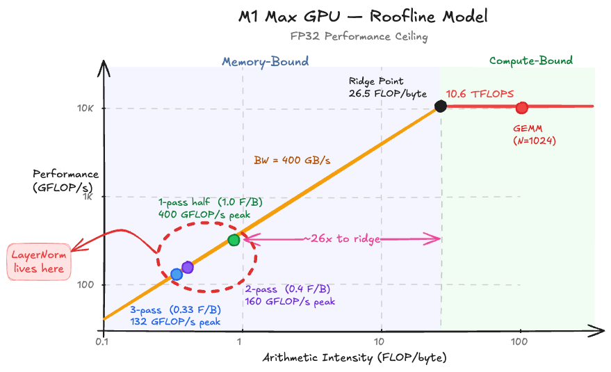
In performance engineering, the ratio of FLOPs to bytes moved is called the arithmetic intensity. It determines whether a kernel is limited by compute or by memory:
To put this in context, the ridge point on Apple Silicon chips (where the roofline transitions from memory-bound to compute-bound) ranges from 26 to 38 FLOP/byte:
| Chip | FP32 TFLOPS | Memory BW (GB/s) | Ridge Point (FLOP/byte) |
|---|---|---|---|
| M1 (8-core) | 2.6 | 68.25 | 38.1 |
| M1 Max (32-core) | 10.6 | 400 | 26.5 |
| M4 (10-core) | 3.8 | 120 | 31.3 |
| M4 Pro (20-core) | 7.5 | 273 | 27.5 |
| M4 Max (40-core) | 15.1 | 546 | 27.6 |
At 0.33–1.0 FLOP/byte, LayerNorm operates at less than 4% of the ridge point on every Apple Silicon chip. It is profoundly memory-bound. Adding more arithmetic won't help. The only thing that matters is how efficiently we move data.
This reframes the optimization goal entirely: we're not trying to reduce FLOPs, we're trying to maximize achieved memory bandwidth — measured as:
The Roadmap
Here's where each kernel lands — the full journey from 5 GB/s to beating PyTorch, with each step motivated by a specific bottleneck in the previous kernel's profile:
| Kernel | Key Optimization | Profiler Motivation | Apple Silicon Insight | BW @ B=8192 (GB/s) |
|---|---|---|---|---|
| K1: Naive | Baseline: 1 thread/row | — | 32 cores, SIMD width 32 | ~5 |
| K2: Coalesced | Threadgroup reduction | Occupancy 0.95%, L1 miss 99.5% | — | ~100 |
| K3: SIMD | simd_sum() replaces tree | Threadgroup barrier stalls | SIMD shuffle BW 2× NVIDIA | ~120 |
| K4: Vectorized | float4 loads | Per-line: Memory Load 45%, 4B each | Native float4 with 16B loads | ~250 |
| K5: 2-pass fused | Device reads = 3× input; min is 2× | SLC keeps 2nd pass warm | ~300 | |
| K6: Welford + half | Single-pass, half4 | Numerical stability; BW ceiling | FP16 = FP32 compute; simd_shuffle_down | ~350+ |
| PyTorch native | (reference) | — | — | ~190 |
Our Profiling Toolkit
In order to benchmark our code and identify bottlenecks, we need a solid profiling toolkit. We will be using different profiling tools to diagnose why a kernel is slow, not just that it's slow. Here's the profiling stack we cover in this blog, introduced progressively as each kernel demands it:
| Question | Tool | Key Metric | Introduced in |
|---|---|---|---|
| How fast is my kernel? | MPS Events (bench_events.py) | GPU-side ms | K1 |
| Is dispatch overhead the problem? | PyTorch Profiler (profile_torch.py) | CPU time vs GPU time | K1 |
| What subsystem is the bottleneck? | Xcode GPU Trace — Limiter tab (gpu_capture.py) | Limiter % per subsystem | K2 |
| Which instructions are expensive? | Xcode GPU Trace — Shader profiler | Per-line cost % | K3 |
| How much memory traffic am I generating? | Xcode GPU Trace — Memory counters | Device Read/Write MiB | K4 |
We capture .gputrace files programmatically through the MTLCaptureManager API, exposed to Python via pybind11. The resulting trace files open in Xcode and show per-kernel occupancy, memory bandwidth utilization, and per-line shader costs. This is Metal's equivalent of CUDA's Nsight Compute, although less automated. We'll introduce each tool in this blog iteratively, when a kernel's specific bottleneck demands it.
torch.profiler doesn't support MPSThe torch.profiler supports ProfilerActivity.CPU and ProfilerActivity.CUDA — but there is no ProfilerActivity.MPS. This has been an outstanding PyTorch feature request since 2023. We can still extract useful CPU-side signals from it (dispatch overhead, back-pressure), but for GPU-side analysis we need Metal's native tools.
K1: A Naive Kernel
Let's start with the most straightforward implementation, directly translating the three mathematical passes into code. One thread handles one entire row in our matrix:
kernel void layernorm_naive(
    device const float*  src   [[buffer(0)]],
    device float*        dst   [[buffer(1)]],
    device const float*  gamma [[buffer(2)]],
    device const float*  beta  [[buffer(3)]],
    constant int64_t&    N     [[buffer(4)]],
    constant float&      eps   [[buffer(5)]],
    uint row [[thread_position_in_grid]])
{
    // Pass 1: compute mean
    float sum = 0.0f;
    for (uint i = 0; i < uint(N); i++)
        sum += src[row * N + i];
    float mean = sum / float(N);

    // Pass 2: compute variance
    float var = 0.0f;
    for (uint i = 0; i < uint(N); i++) {
        float diff = src[row * N + i] - mean;
        var += diff * diff;
    }
    float scale = rsqrt(var / float(N) + eps);

    // Pass 3: normalize with affine transform
    for (uint i = 0; i < uint(N); i++)
        dst[row * N + i] = (src[row * N + i] - mean) * scale * gamma[i] + beta[i];
}
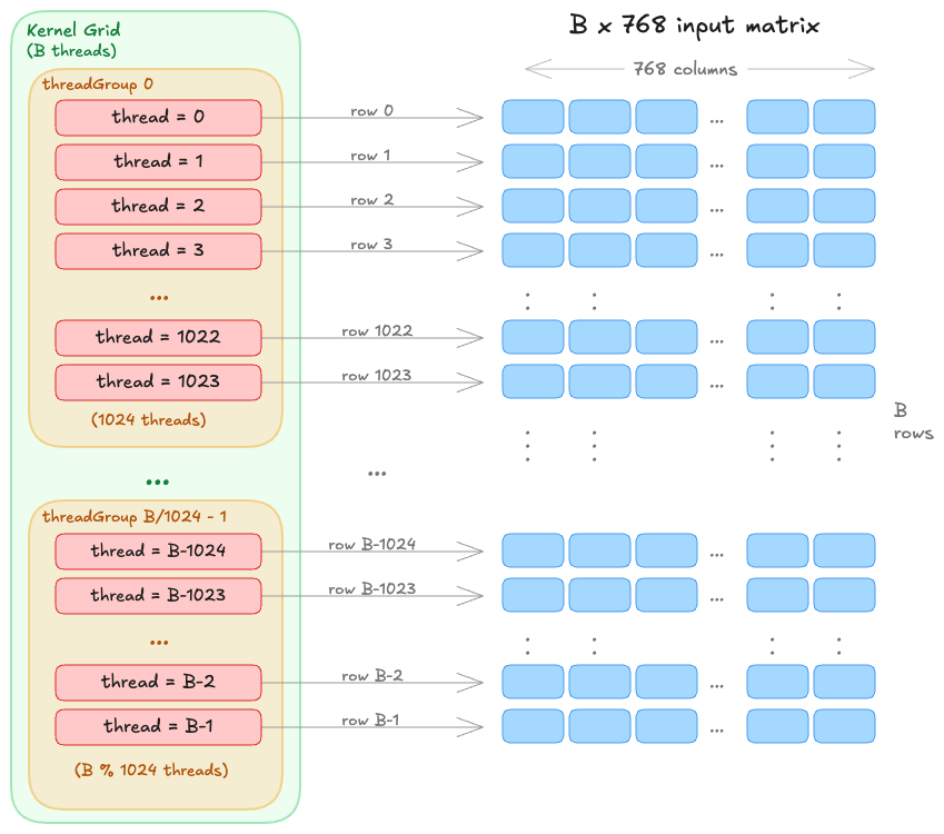
The kernel dispatch maps one thread per row for a grid size (B, 1, 1). Each thread independently reads its row three times, computes the statistics, and writes the normalized output.
MTLSize gridSize = MTLSizeMake(B, 1, 1);
NSUInteger tgWidth = std::min(
    (NSUInteger)B, pso.maxTotalThreadsPerThreadgroup);
tgWidth = std::min(tgWidth, (NSUInteger)1024);
MTLSize tgSize = MTLSizeMake(tgWidth, 1, 1);
[enc dispatchThreads:gridSize threadsPerThreadgroup:tgSize];
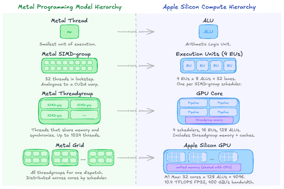
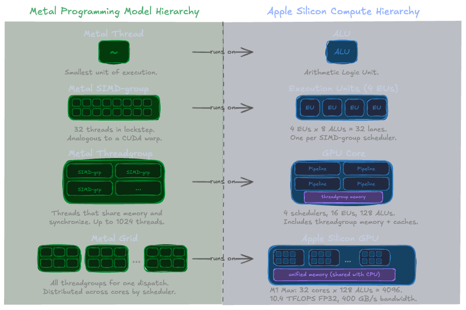
Mapping Metal's Programming Model to Apple Silicon Compute Hierarchy (👉 expand)
Benchmarking with MPS Events
To find out how fast our kernel is, we need to measure actual GPU execution time. The way to time Metal kernels is with MPS Events, which record timestamps directly on the Metal command queue (measuring actual GPU execution time, not CPU dispatch overhead).
start = torch.mps.event.Event(enable_timing=True)
end   = torch.mps.event.Event(enable_timing=True)

start.record()
for _ in range(NUM_ITERS):
    _ = layernorm_forward(x, gamma, beta, eps, kernel="naive")
end.record()
torch.mps.synchronize()

elapsed_ms = start.elapsed_time(end) / NUM_ITERS
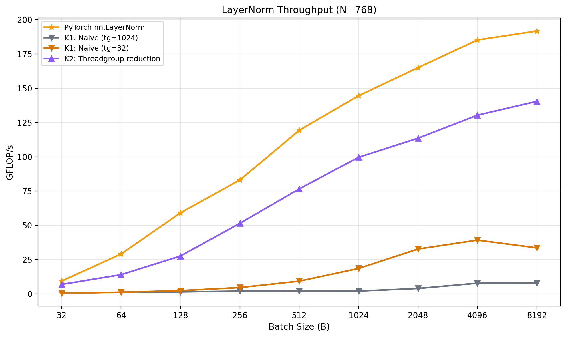
I benchmarked our naive kernel against PyTorch's native torch.nn.functional.layer_norm across a sweep of batch sizes at N=768 (GPT-2's hidden dimension), FP32, on my M1 Max:
 MPS event timing, 10 warmup + 100 measured iterations.
Our naive kernel is between 23× (B=8192) and 40× (B=256) slower than PyTorch. Not surprising for a first attempt, but the magnitude of the gap is telling. At B=8192, our kernel achieves roughly 5 GB/s of memory bandwidth i.e. about 1% of the M1 Max's 400 GB/s peak. We established in the roofline analysis that LayerNorm is profoundly memory-bound, so bandwidth is the only metric that matters. 1% utilization means we're not just slow, we're barely using the hardware at all. Why?
K1 Bottleneck: Uncoalesced Memory Access
Look back at the dispatch geometry: dispatchThreads:{B, 1, 1} with one thread per row. Threads in the same SIMD group (Metal's equivalent of a CUDA warp, made up 32 threads that execute in lockstep) utilize common underlying memory access hardware. The hardware (ideally) wants to see 32 adjacent threads reading 32 adjacent addresses so it can coalesce (combine) them into one or two wide memory transactions. However, in our naive kernel we are processing different rows in each thread. In the physical device memory, the matrix is stored in a linear, row-major fashion. When the SIMD group issues a memory load, thread 0 reads src[i+0], thread 1 reads src[i+768], thread 2 reads src[i+1536], and so on per each iteration in our loop. Each of these address is separated by N×4 = 3072 bytes. The memory controller fetches data in 128-byte cache lines, so each of these 32 threads triggers a fetch to a different cache line. Instead, we are essentially issuing 32 independent fetches scattered across memory.
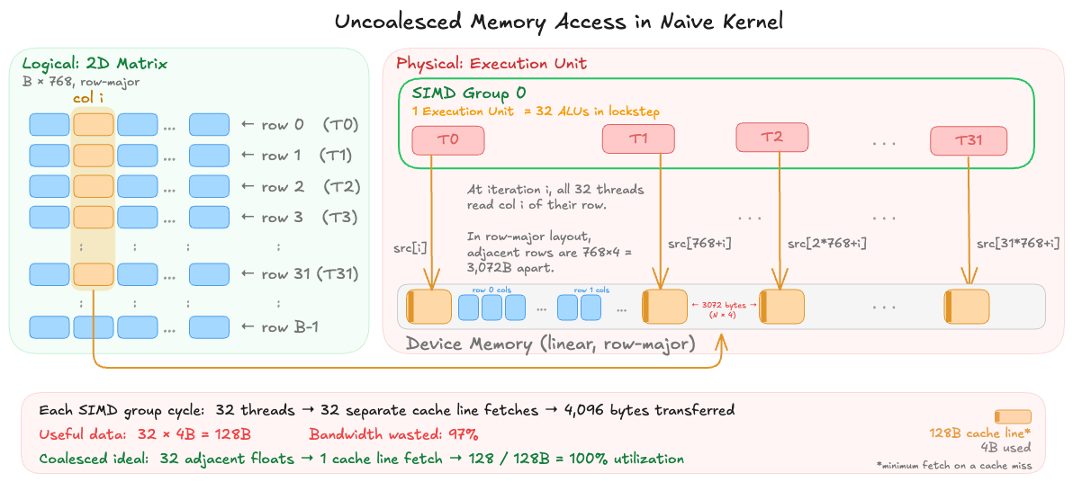
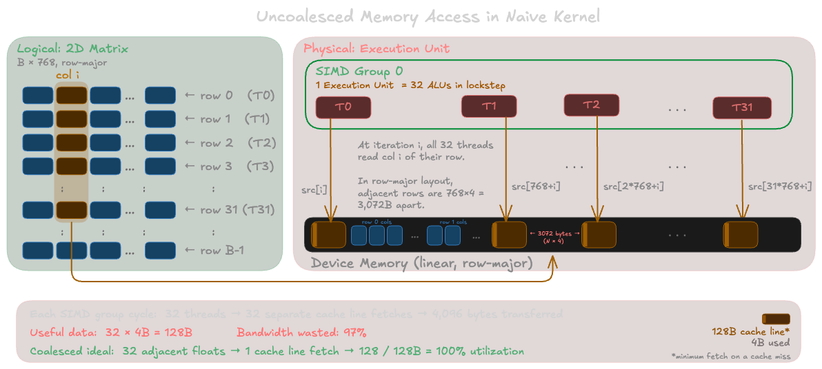
This is the classic uncoalesced access pattern, and it has two compounding effects. First, the memory bus is massively underutilized. Instead of saturating a 128-byte transaction with 32 useful floats, we're loading 128 bytes to extract a single 4-byte float, wasting 97% of each fetch operation. Second, the L1 cache (which is per-core, only 8 KB on Apple Silicon) thrashes immediately: the 32 fetched cache lines evict each other before any thread can reuse them on the next loop iteration.
There's a secondary problem layered on top: occupancy. Our dispatch creates B threads in a single 1D grid. At B=1024, that's one threadgroup of 1024 threads on one GPU core — while the other 31 cores on the M1 Max sit completely idle. Even if the memory access pattern were perfect, we'd be limited to 1/32 of the chip's bandwidth.
K1b: An Ablation on Occupancy
Still Naive, but hiding latency with occupancy
We can isolate the occupancy effect with a one-line experiment: change tgSize from 1024 to 32.
NSUInteger maxTg = (kernel_name == "layernorm_naive_32")
                   ? (NSUInteger)32 : (NSUInteger)1024;
This doesn't touch the kernel code or fix the access pattern, each thread still processes one row, and adjacent threads in a SIMD group still read strided addresses. But at B=1024, we now get 32 threadgroups instead of 1, spreading work across all 32 GPU cores. The memory access pattern is still terrible, but with 32× more SIMD groups in flight, the memory controller has more outstanding requests to overlap — when one group stalls on a cache miss, another can issue its own requests. This is pure latency hiding through parallelism.
 MPS event timing, 10 warmup + 100 measured iterations, N=768, FP32, M1 Max.
The results confirm that occupancy alone helps but doesn't come close to solving the problem. At B=1024, where the effect is cleanest (1 vs 32 threadgroups), tg=32 achieves a 9× speedup — from 6 GB/s to 55 GB/s. But 55 GB/s is still just 14% of the M1 Max's 400 GB/s peak, and PyTorch is at 366 GB/s. The uncoalesced access pattern wastes so much of every memory transaction that even 32 cores issuing requests in parallel can't compensate.
Two details in the data are worth highlighting.
- At B=32,
tg=32gives exactly 1 threadgroup, the same astg=1024, so there's no improvement. This is the control: same kernel, same threadgroup count, same performance, confirming that the threadgroup size parameter itself isn't affecting anything beyond the number of groups. tg=32peaks at B=4096 (117 GB/s) and then drops to 102 GB/s at B=8192. At B=8192, the input tensor is 24 MiB; with 256 threadgroups all issuing scattered cache line fetches, the LLC (Last Level Cache) is under heavy churn from the strided access pattern. More parallelism actually worsens cache contention once the working set is large enough.
While these are both problems that GPU programmers can diagnose from seeing the code alone, let's see if we can work them out from profiling. Along the way, we will also build the profiling workflow we'll use for every subsequent kernel. For optimizing memory-aware algorithms, even experts (like PyTorch devs) often rely on profiling results over theoretical intuition:
this is why we profile and don’t just rely on intuition…
— Daniel Vega-Myhre (@vega_myhre) March 5, 2026
What torch.profiler Reveals (and Doesn't)
If you're coming from CUDA, your first instinct for profiling is probably torch.profiler. It integrates with Perfetto UI, supports record_shapes for tracking tensor dimensions, and can capture Python call stacks. It also doesn't support MPS (whomp, whomp).

But the CPU profiler can still reveal useful signals. Running it on PyTorch's native LayerNorm (B=1024, N=768) we find:
native_layer_norm allocates three output tensors: the normalized result, plus the per-row mean and reciprocal standard deviation. These intermediate statistics are returned for the backward pass (more on this later).
However, the more interesting signal from the CPU profiler is what happens to dispatch time across the 100-iteration run. When we zoom out, PyTorch's native LayerNorm stays at a flat ~5–6 µs across all 100 iterations during our CPU profiling: no inflation, no back-pressure. Now, let's compare this to our naive kernel:
For the first ~10 iterations, the CPU enqueues work into the MPS command buffer faster than the GPU can drain it, so dispatch_sync returns immediately after encoding. At iteration 10, the buffer fills and the dispatch call blocks until the GPU completes a kernel — the 939 µs spike is the first time the CPU waits on the GPU. The escalation to ~3 ms in later iterations reflects the accumulated back-pressure from our slow naive kernel.
| Iterations | pybind11 C++ dispatch (µs) | Interpretation |
|---|---|---|
| 0–9 | ~10 | CPU races ahead — pure encode + commit overhead |
| 10 | 939 | Command buffer saturates, CPU blocks for the first time |
| 11–50 | ~75–90 | Steady-state back-pressure from slow GPU execution |
| 80–99 | ~3,000 | Heavy back-pressure — GPU can't keep up |
The CPU profiler is indirectly revealing GPU performance: the dispatch time inflates because the CPU is being throttled by the GPU. But that back-pressure signal is crude. It tells us the GPU is slow, not why. For that, we need to look inside the kernel.
Detour: CPU-side warmup effects, profiler insights, and a dispatch overhead fix
Both traces show significant first-iteration overhead. PyTorch's aten::layer_norm takes 83 µs on the first call versus ~6 µs at steady state — the cost concentrates in aten::empty_like (10.7 µs vs ~0.6 µs) and aten::empty (8.2 µs vs ~0.2 µs), consistent with MPS buffer pool initialization and Metal pipeline state compilation on the first pass.
Our naive kernel's first iteration told a more interesting story. Looking at the per-iteration breakdown in the original trace:
wrapper.py: layernorm_forward              (~38 µs steady-state)
├── wrapper.py: _shader_path               (~27 µs)  ← pkg_resources filesystem walk
│   └── pkg_resources.resource_filename
└── pybind11: layernorm_forward            (~10 µs)   ← C++ dispatch → Metal
    └── aten::empty_like [1024, 768]       (~1.5 µs)
        └── aten::empty_strided            (~0.7 µs)
The _shader_path() function called pkg_resources.resource_filename() on every invocation — which internally constructs a NullProvider object, walks parent directories via _parents() (called 6 times per invocation), and checks each for egg/zip paths. The CPU profiler trace ballooned to 14,333 events, with 3,500 of them from pkg_resources alone — all for a path that never changes. The ~27 µs of Python filesystem overhead per call made our wrapper dispatch ~7× more expensive than PyTorch's native path.
The fix: add @lru_cache so the filesystem walk happens once per shader file instead of once per kernel invocation:
from functools import lru_cache

@lru_cache(maxsize=None)
def _shader_path(filename: str) -> str:
    return pkg_resources.resource_filename(
        'layernorm_metal', f'kernels/{filename}'
    )
With 8 kernel variants in the KERNELS dict, that's at most 8 cached entries. I fixed this in this commit and re-profiled. The before/after comparison:
| Metric | Before (no cache) | After (lru_cache) |
|---|---|---|
| Total trace events | 14,333 | 733 |
pkg_resources events | 3,500 | 0 |
_shader_path per call | ~27 µs | <1 µs (invisible to profiler) |
layernorm_forward wrapper (steady-state) | ~38 µs | ~15 µs |
| Wrapper → pybind11 gap | ~27 µs | ~0.3 µs |
And the per-iteration dispatch times with warmup:
| Iteration | PyTorch native (µs) | Our kernel, before (µs) | Our kernel, after (µs) |
|---|---|---|---|
| 0 | 83.4 | 182.0 | 119.2 |
| 1 | 8.2 | 48.5 | 33.8 |
| 2 | 6.7 | 41.4 | 15.5 |
| 5 | 6.3 | 36.5 | 13.0 |
| 9 | 5.8 | 38.2 | 20.1 |
The wrapper now adds essentially zero overhead on top of the pybind11 C++ dispatch. Meanwhile, the GPU back-pressure pattern is unchanged as iteration 10 still spikes to 933 µs, iterations 80–99 still hit ~3,100 µs. This confirms that the overhead was purely CPU-side and doesn't affect our MPS-event-timed GPU benchmarks. However, it matters for end-to-end latency at small batch sizes where CPU dispatch is a larger fraction of wall-clock time.
Introducing GPU Capture
Metal's MTLCaptureManager API lets us programmatically record a .gputrace file containing every command buffer, encoder call, and hardware performance counter. We expose the capture start/stop calls through pybind11 in dispatch.mm:
void start_gpu_capture(const std::string& output_path) {
    id<MTLDevice> device = getPipelineCache().getDevice();
    MTLCaptureManager* mgr = [MTLCaptureManager sharedCaptureManager];

    if (![mgr supportsDestination:MTLCaptureDestinationGPUTraceDocument]) {
        TORCH_CHECK(false,
            "GPU trace capture not supported. "
            "Set METAL_CAPTURE_ENABLED=1 before launching Python.");
    }

    NSString* nsPath = [NSString stringWithUTF8String:output_path.c_str()];
    [[NSFileManager defaultManager] removeItemAtPath:nsPath error:nil];

    MTLCaptureDescriptor* desc = [[MTLCaptureDescriptor alloc] init];
    desc.captureObject = device;
    desc.destination = MTLCaptureDestinationGPUTraceDocument;
    desc.outputURL = [NSURL fileURLWithPath:nsPath];

    NSError* error = nil;
    BOOL ok = [mgr startCaptureWithDescriptor:desc error:&error];
    TORCH_CHECK(ok, "Failed to start GPU capture: ",
                error.localizedDescription.UTF8String);
}

void stop_gpu_capture() {
    [[MTLCaptureManager sharedCaptureManager] stopCapture];
}
The capture targets the MTLDevice itself, which means it records all command buffers submitted to that device between start and stop. The METAL_CAPTURE_ENABLED=1 environment variable must be set before launching Python, as Metal disables the capture API by default for security.
METAL_CAPTURE_ENABLED=1 python benchmarks/gpu_capture.py -k naive_1024 --B 1024 --num-iters 10
open /tmp/layernorm_naive_1024.gputrace
Opening the trace in Xcode shows the GPU Debugger landing view:
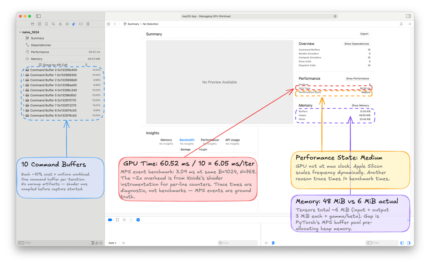
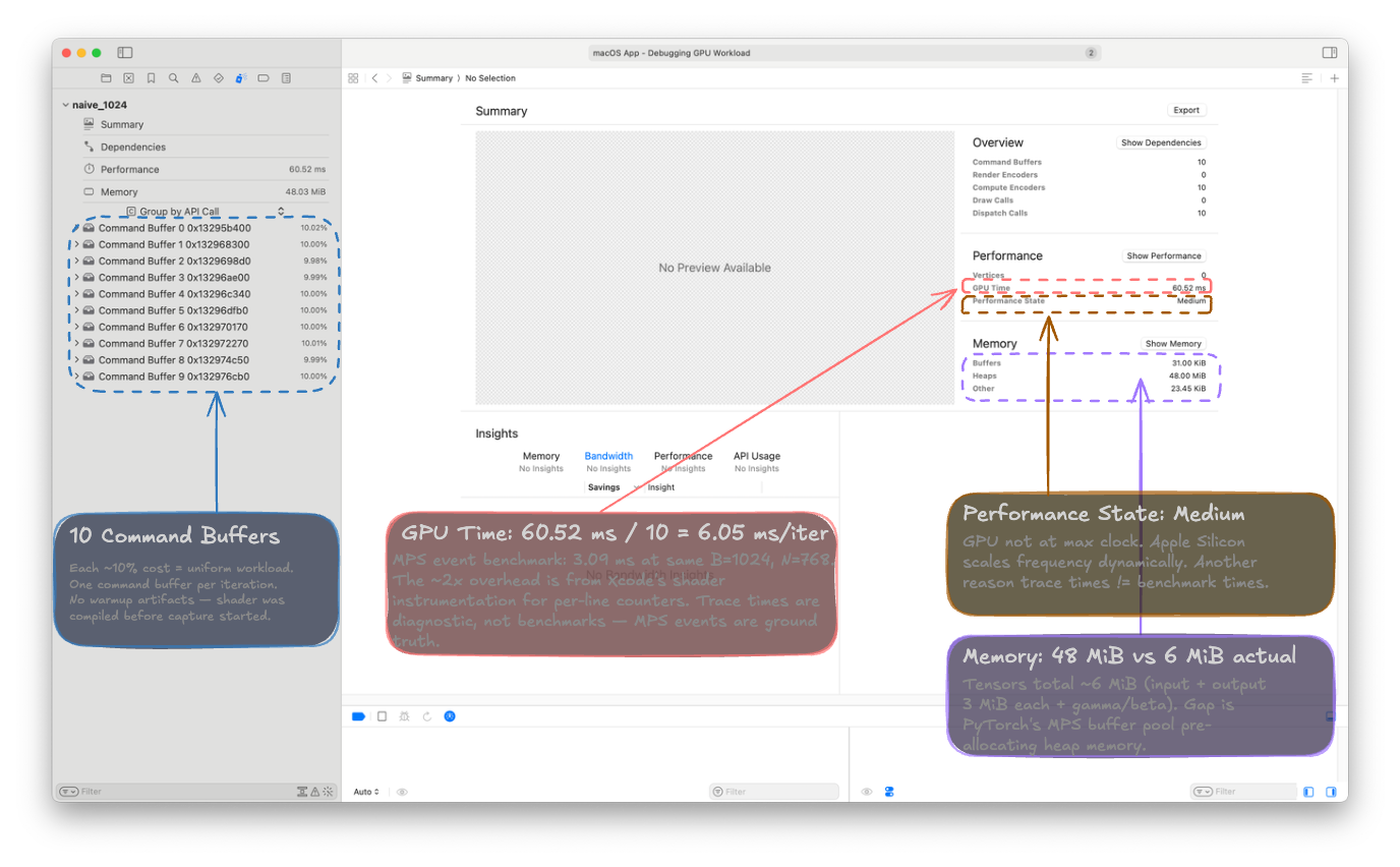
A few things to note: 10 Command Buffers, ~10% each (one per iteration, uniformly distributed). GPU Time: 60.52 ms total = 6.05 ms per iteration, roughly 2× our MPS event measurement due to Xcode's shader instrumentation overhead. Trace times are diagnostic, not benchmarks. MPS events remain the source of truth for absolute timing.
Command Buffer Hierarchy (👉 expand)
Expanding a single command buffer in the left sidebar reveals the full dispatch sequence. Every entry maps directly to an Objective-C call in dispatch.mm:
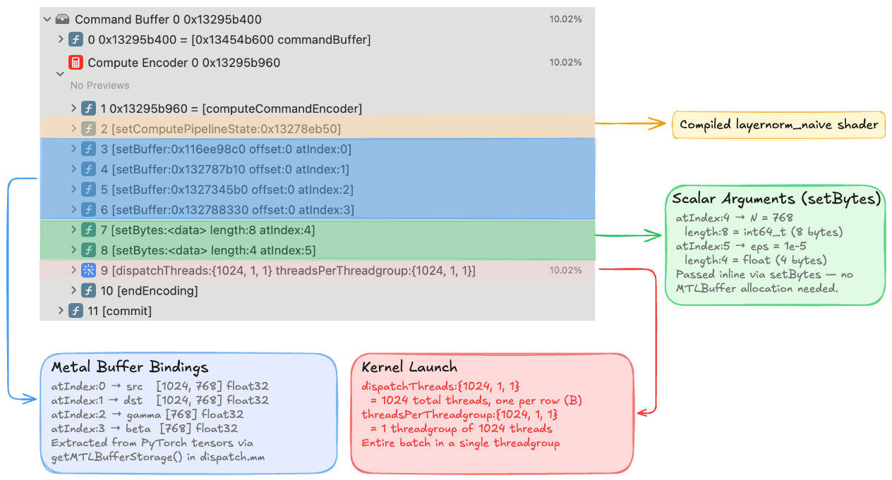
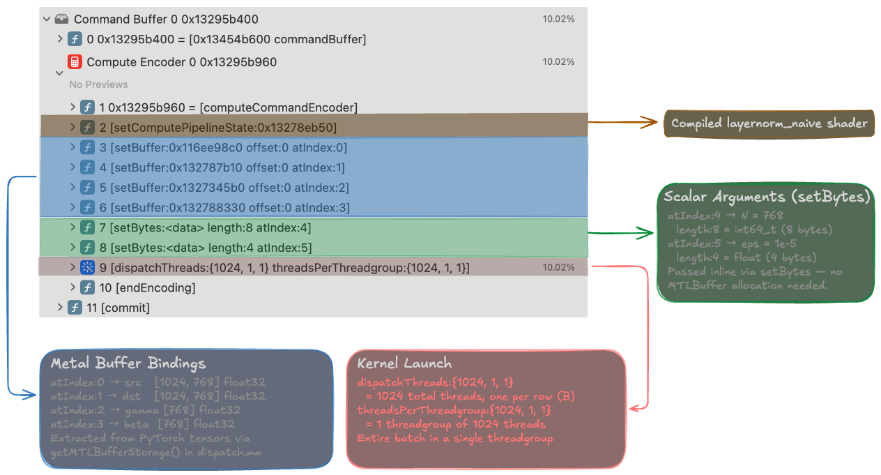
The four setBuffer calls at indices 0–3 bind the Metal buffers we extracted from PyTorch tensors via getMTLBufferStorage(), mapping directly to the kernel signature:
kernel void layernorm_naive(
    device const float*  src   [[buffer(0)]],   // setBuffer atIndex:0
    device float*        dst   [[buffer(1)]],   // setBuffer atIndex:1
    device const float*  gamma [[buffer(2)]],   // setBuffer atIndex:2
    device const float*  beta  [[buffer(3)]],   // setBuffer atIndex:3
    constant int64_t&    N     [[buffer(4)]],   // setBytes length:8 (int64)
    constant float&      eps   [[buffer(5)]],   // setBytes length:4 (float)
    uint row [[thread_position_in_grid]])
The two setBytes calls at indices 4–5 pass scalar arguments inline — length:8 for the 8-byte int64_t N=768, and length:4 for the 4-byte float eps=1e-5. Finally, dispatchThreads:{1024, 1, 1} threadsPerThreadgroup:{1024, 1, 1} dispatches 1024 threads (one per row, matching B=1024) in a single threadgroup.
The Performance->Timeline view shows events as they happened on the GPU:
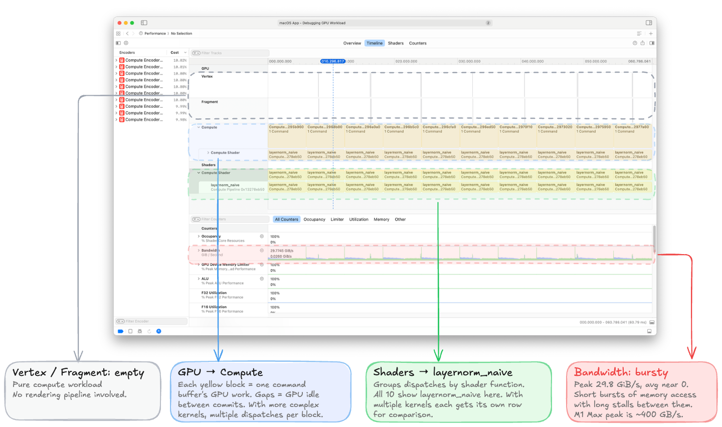
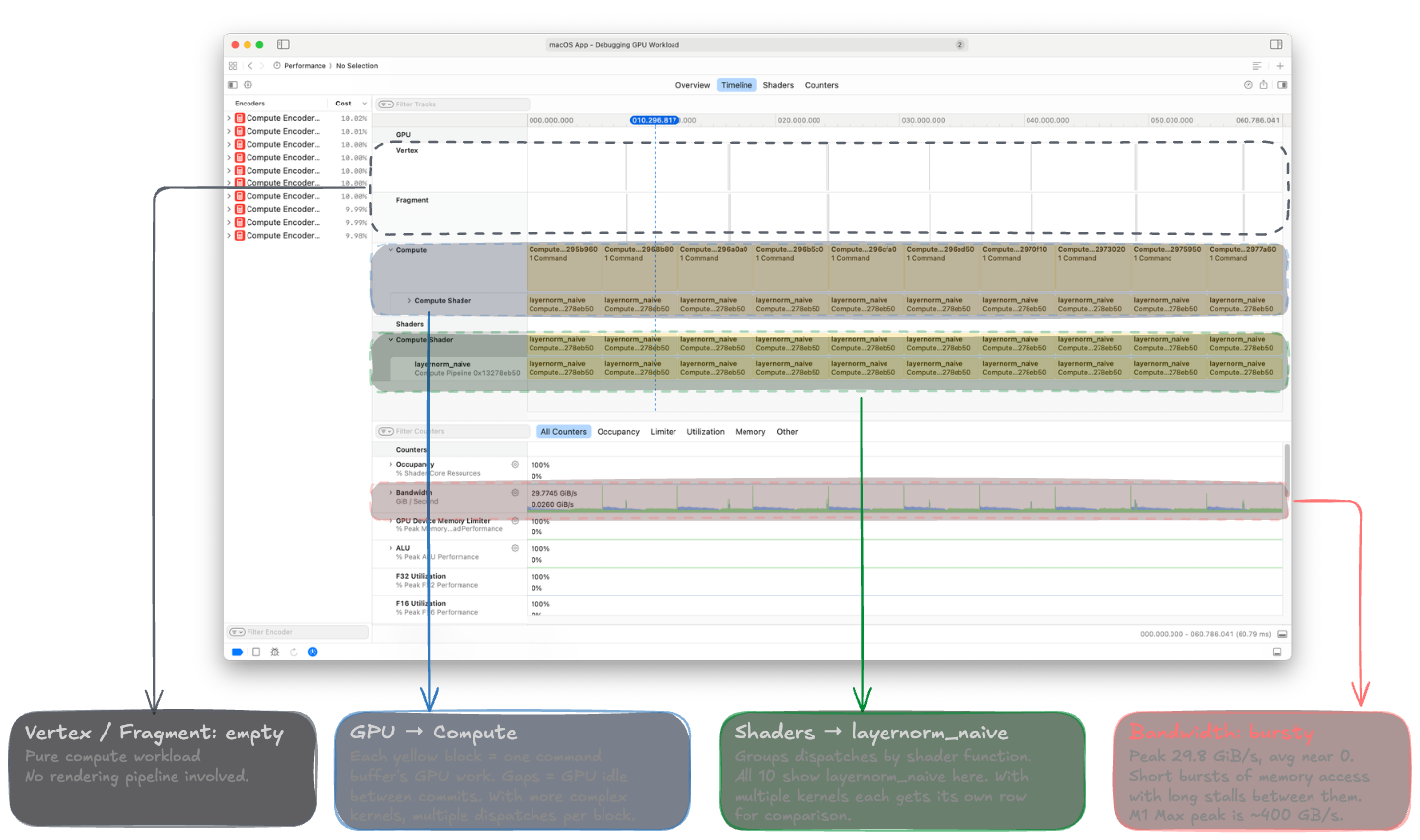
 Even at a glance, one counter stands out: Bandwidth peaks at 29.8 GiB/s but averages near zero, forming a spiky pattern with short bursts of memory activity separated by long idle periods.
Performance Counter Driven Diagnostics
We will introduce the remaining two performance sections (Shaders and Counters) progressively as we optimize our kernel. Rather than dump every performance counter for K1, I will mention three numbers that tell the complete story:
Kernel Occupancy: 0.95%. The dispatch creates exactly one threadgroup of 1024 threads. On the M1 Max with 32 GPU cores, that single threadgroup runs on one core while the other 31 sit completely idle.
Buffer L1 Miss Rate: 99.54%. Essentially every L1 cache access misses. Thread 0 reads src[0], thread 1 reads src[768], thread 2 reads src[1536] — each in a completely different cache line. The L1 provides zero reuse. This drives a 16× LLC traffic amplification: 146 MiB of LLC reads to satisfy 9 MiB of DRAM reads.
Achieved Bandwidth: ~5 GB/s out of 400 GB/s peak — roughly 1% utilization.
We already covered the theoretical intuition for these numbers in the Benchmarking with MPS Events section. The GPU profiler confirms our diagnosis: the kernel is bottlenecked by uncoalesced memory access and poor occupancy, leading to a massively underutilized memory subsystem. It's good to know that we can derive these insights from the profiler, because for more complex kernels intuition alone won't be enough to identify bottlenecks.
K2: Coalesced Memory Access + Threadgroup Tree Reduction
K1 had two problems: uncoalesced access (adjacent threads reading different rows) and poor occupancy (one threadgroup on one core). K2 fixes both by restructuring so that one threadgroup processes each row:
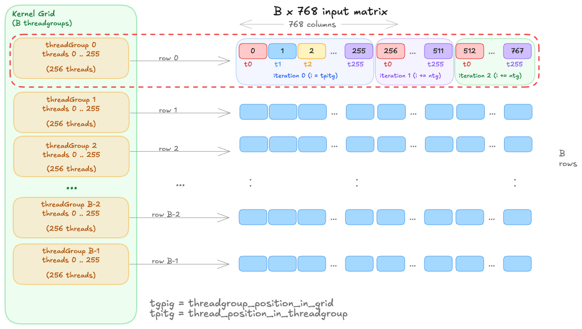
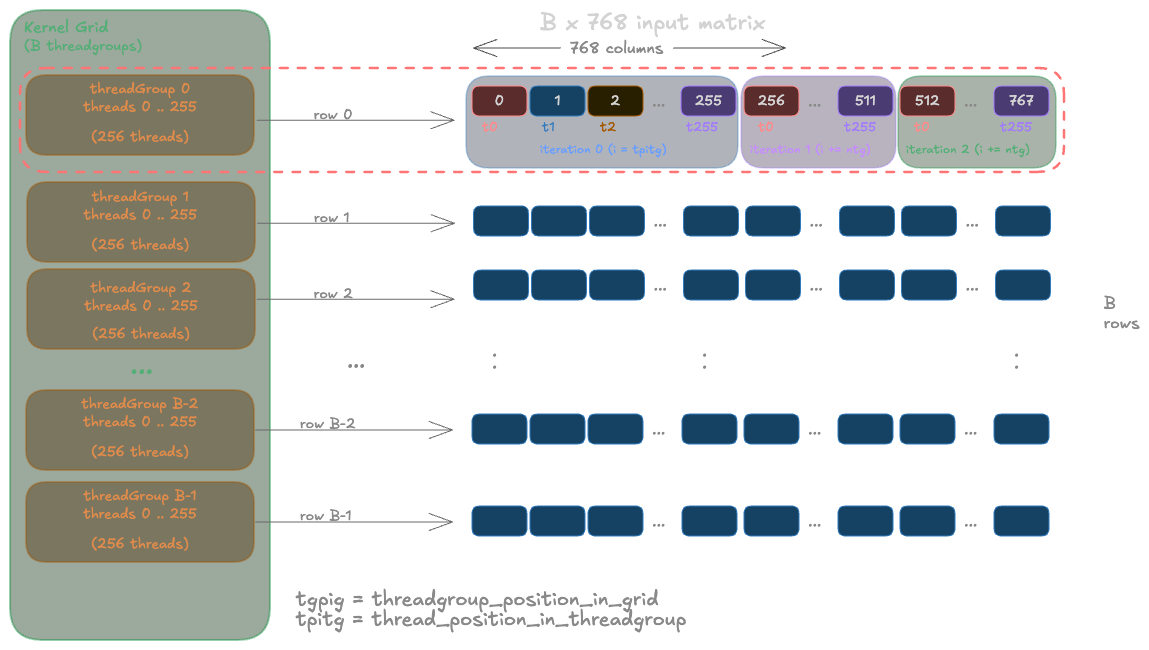
By assigning a threadgroup to a row, we allow adjacent threads to read adjacent elements in memory (coalesced). Depending on the size of the threadgroup and batch B, each thread can read one or more elements in a strided pattern and accumulate the results (e.g. each thread reads 3 elements of a row in the image shown). But the key advantage is that the threads in a SIMD group will now be reading from the same cache line, allowing the memory controller to coalesce their requests into fewer transactions.
kernel void layernorm_shared(
    ...
    threadgroup float*   buf   [[threadgroup(0)]],
    uint tgpig [[threadgroup_position_in_grid]],   // row index
    uint tpitg [[thread_position_in_threadgroup]],  // thread within row
    uint   ntg [[threads_per_threadgroup]])
{
    device const float* row_src = src + tgpig * N;

    // Coalesced load: consecutive threads read consecutive elements
    float local_sum = 0.0f;
    for (uint i = tpitg; i < uint(N); i += ntg)
        local_sum += row_src[i];

    // Tree reduction in threadgroup memory
    buf[tpitg] = local_sum;
    threadgroup_barrier(mem_flags::mem_threadgroup);
    for (uint stride = ntg / 2; stride > 0; stride /= 2) {
        if (tpitg < stride)
            buf[tpitg] += buf[tpitg + stride];
        threadgroup_barrier(mem_flags::mem_threadgroup);
    }
    float mean = buf[0] / float(N);
    // ... repeat for variance, then normalize ...
}
Once each thread in the threadgroup has computed its local sum, we move the partial sums into threadgroup memory (which all threads in the group can access). We then perform a tree reduction: log₂(ntg) rounds of pairwise addition, with a threadgroup_barrier() between each round to ensure all writes are visible before the next round reads. The same pattern is repeated for variance, and then we normalize in-place using the computed mean and variance.
For the more visual learners, here is a breakdown of the code above into steps showing memory copy, accumulation, and reduction operations. You can also see the memory view of the operations in the memory hierarchy tab.
The tree reduction requires the threadgroup size to be a power of 2 (each round halves the active threads). Our dispatch code rounds ntg down to the nearest power of 2: for N=768, this gives ntg=512, not 768. Some threads handle 2 elements in the accumulation loop while others handle 1. We will see how to work around this constraint later.
How well does K2 perform?
By recording with mps.event, we find that the memory bandwidth jumps from ~5 to ~100 GB/s, a nearly 20× improvement and the massive absolute gain in the entire progression. But we're still only at roughly 25% of the M1 Max's 400 GB/s peak. For K1, we diagnosed the bottleneck from the code and confirmed it with three headline numbers from the profiler. K2 looks reasonable — coalesced loads, parallel reduction, full core occupancy. So the bottleneck may not be obvious from the code alone. From here on, we will let the profiler take the lead.
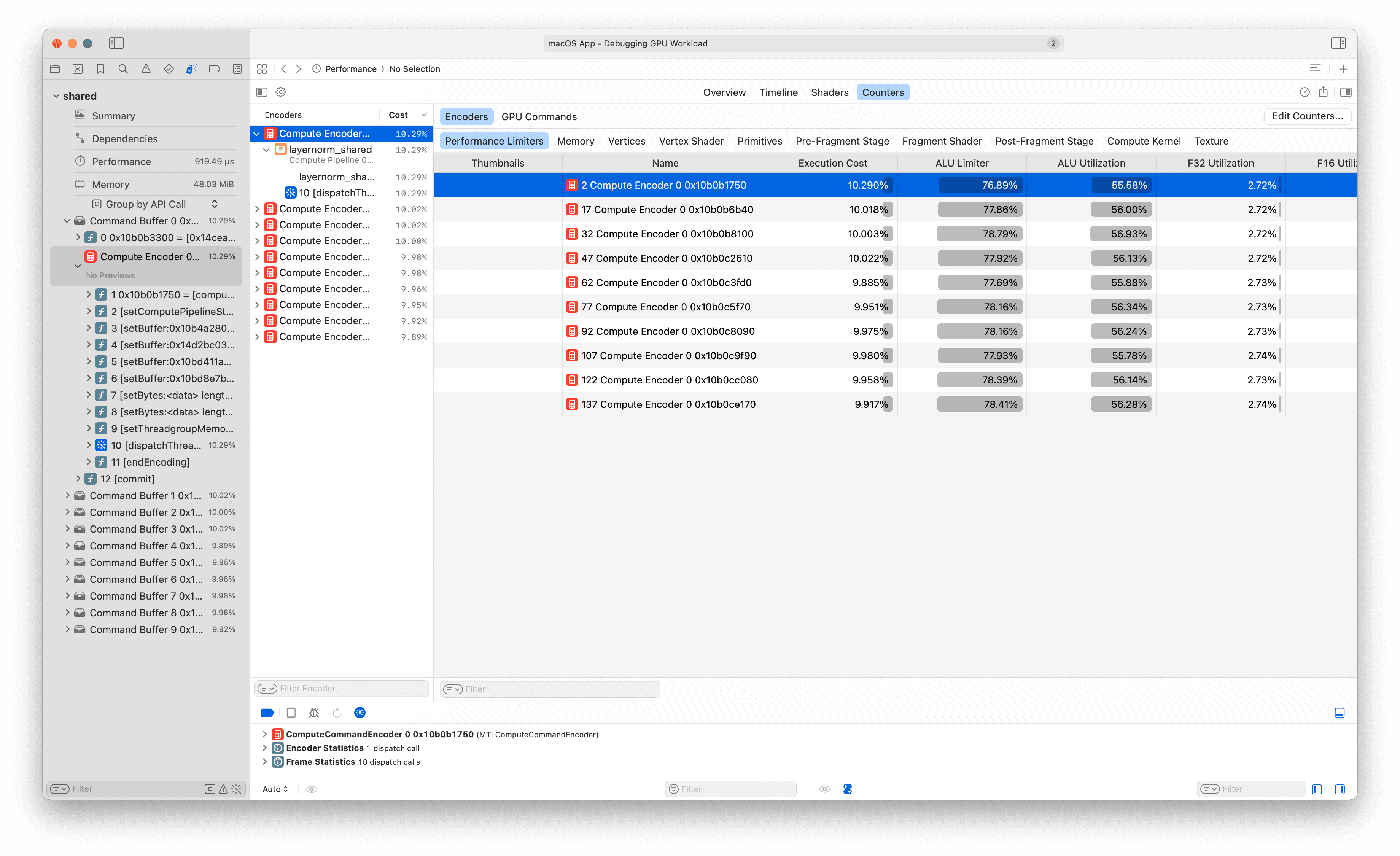
Profiler: Introducing the Counters Tab
It's time to introduce a new profiling tool in our XCode gputrace toolkit. Select any single compute encoder in Xcode's left sidebar, then switch to the Performance->Counters tab at the top. This gives exact per-subsystem Limiter percentages (fraction of time the GPU stalled waiting on each subsystem), Utilization percentages (fraction of peak throughput achieved), and memory traffic totals.
For K1 we only used three headline numbers because the GPU was so underutilized that the detailed counters were all near zero. K2 is different: the GPU is busy, and the counters have more information to convey.
What K2 fixed
First, the good news. The counters confirm that our two K1 problems, occupancy and memory access, are both dramatically improved:
| Counter | K1 | K2 | What changed |
|---|---|---|---|
| Kernel Occupancy | 0.95% | 84.90% | 1 → 1024 threadgroups across 32 cores |
| Device Memory Read | 9.08 MiB | 3.28 MiB | LLC serves repeat passes; DRAM reads ≈ 1× input |
| LLC Read Traffic | 146.20 MiB | 14.12 MiB | Coalesced access eliminates cache line thrashing |
| Device Memory Bandwidth | 0.52 GiB/s | 17.8 GiB/s | 34× improvement |
The LLC traffic collapse is the most striking number: 146 MiB → 14 MiB, a 10× reduction. K1's uncoalesced access pattern caused massive cache line churn, 146 MiB of LLC reads to satisfy 9 MiB of actual data. K2's coalesced accesses stay within cache lines, so the LLC works as intended.
Even more interesting: device memory reads dropped from 9 MiB to 3.28 MiB, which is essentially 1× the input tensor (B=1024 × N=768 × 4 bytes = 3.0 MiB). Our kernel reads X three times (mean, variance, normalize), so the theoretical device memory traffic should be 9 MiB. But the LLC is serving the second and third passes from cache. This is Apple Silicon's 48 MB System Level Cache (SLC) at work, which sits between the GPU cores and DRAM, it's 8× larger than the RTX 3090's 6 MB L2 cache (the same-generation NVIDIA consumer GPU). At this batch size, our entire input fits in the SLC, so the second and third passes read at SLC bandwidth rather than DRAM bandwidth. On the 3090, the same input would be 4× larger than L2, and every pass would hit DRAM. We'll quantify this SLC advantage more carefully in K4, where it explains how our kernel measures bandwidth above the DRAM peak.
Why is the Buffer L1 miss rate still 94.55%? (👉 expand)
We fixed coalescing, so why does L1 still miss at nearly the same rate as K1 (99.54%)? The miss rate is misleading here — what changed is the miss cost. In K1, each miss pulled in a cache line where only 4 of 128 bytes were useful (3% utilization per fetch). In K2, each miss pulls in a cache line where all 128 bytes are used by adjacent threads in the SIMD group.
The L1 still misses frequently because of occupancy-driven cache pressure: with 84.9% occupancy, roughly 32 threadgroups share each core's 8 KB L1. Each threadgroup's working set is ~3 KB (768 × 4 bytes), so the aggregate demand per core (~96 KB) is 12× larger than the L1. The cache thrashes from inter-threadgroup contention, not from bad access patterns. But the LLC catches these misses efficiently — that's why device memory reads are just 3.28 MiB despite the 94% L1 miss rate.
So, what's the new bottleneck?
Here are the counters that grew from K1 to K2:
| Counter | K1 | K2 |
|---|---|---|
| ALU Limiter | 0.12% | 76.89% |
| Integer and Complex Limiter | 0.16% | 24.66% |
| LLC Limiter | 5.07% | 29.80% |
| ThreadGroup Read Limiter | 0.00% | 3.03% |
| ThreadGroup Write Limiter | 0.00% | 1.95% |
| ALU Inefficiency | 0.01% | 10.34% |
ALU is the dominant limiter at 77%. For a kernel we established is profoundly memory-bound, this is not what I expected. My initial hypothesis was that threadgroup memory barriers would be the bottleneck (we'll discuss these in a second), but the threadgroup limiters are only 3–5%.
One might assume the 77% ALU limiter means the kernel is now compute-bound: we optimized memory access so well that the arithmetic itself became the ceiling. But a second counter rules that out: F32 Utilization is only 2.72%. The floating-point units that compute actual LayerNorm arithmetic are nearly idle. The ALU is 77% busy, but almost none of that is float math.
The kernel-level ALU breakdown confirms this: 74.5% of all ALU instructions are integer-and-conditional (comparisons, branches, index arithmetic), another 10.5% are integer-and-complex (shifts, multiplies for address computation), and only 4.67% are float. The kernel is overwhelmingly executing reduction bookkeeping, not LayerNorm math.
The other counter worth noting is ALU Inefficiency: 10.34%, up from 0.01% in K1. This measures wasted work from SIMD divergence i.e. threads in the same SIMD group that are masked off because they took a different branch. K1 had zero divergence because every thread ran identical loops.
K2's tree reduction introduces divergence at the if (tpitg < stride) check: in each round, half the threads are active and half are masked off, yet all of them still occupy SIMD lanes and consume scheduling resources.
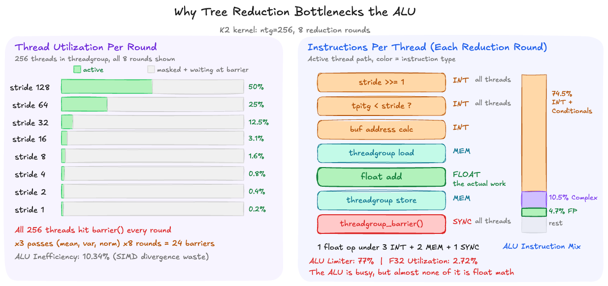
Why the tree reduction dominates ALU
The log₂(ntg) reduction loop looks simple in the source, but each round compiles down to several integer ALU instructions and synchronization operations. With ntg=256, each reduction runs 8 rounds. In each round, the kernel:
- Shifts the stride (
stride /= 2): an integer shift instruction - Compares thread index to stride (
tpitg < stride): an integer comparison - Computes addresses into the threadgroup buffer: integer multiply + add
- Active threads read from threadgroup memory, add, and write back
- All 512 threads hit
threadgroup_barrier(): even the ones that did no useful work
The barrier forces every thread in the threadgroup to synchronize, regardless of whether it participated in the round. By round 8, one thread is doing a single float addition while 255 threads wait. Multiply by 3 reduction passes per row (mean, variance, normalize), and the kernel executes 24 barrier-synchronized rounds per row, each generating shift, comparison, and address-calculation instructions for every thread.
The threadgroup memory traffic tells the same story from a different angle: K2 reads 8.1 MiB and writes 8.0 MiB of threadgroup memory (16 MiB total) compared to 3.28 MiB of actual device memory reads. The tree reduction generates 5× more on-chip traffic than the kernel's real data movement from DRAM.
Apple Silicon's SIMD-first architecture
The counter data reveals that the tree reduction pattern — standard on CUDA where shared memory is fast and cheap — is working against Apple Silicon's hardware. The bottleneck isn't threadgroup memory bandwidth (its limiter is only 3–5%); it's the volume of integer instructions, barriers, and SIMD divergence that log₂(ntg) rounds generate.
This turns out to be by design. Apple made a deliberate architectural tradeoff: reduced threadgroup memory bandwidth in favor of industry-leading SIMD shuffle bandwidth. Philip Turner's metal-benchmarks documents this: SIMD shuffles achieve 256 bytes/cycle — 2× NVIDIA's 128 bytes/cycle. On CUDA, shared memory is the default reduction primitive. On Metal, the hardware is telling us to look elsewhere — specifically, at the SIMD group intrinsics we haven't used yet.
K3: SIMD-First Reduction
K2's bottleneck was the tree reduction: log₂(ntg) rounds of barriers, integer index math, and SIMD divergence — 77% ALU limiter for a kernel where float arithmetic accounts for under 5% of instructions. The hardware is spending most of its time coordinating threads, not computing LayerNorm. We need a reduction that costs essentially zero ALU and zero barriers.
TODO TODO TODO TODO
Metal provides exactly this. simd_sum() is a single intrinsic that reduces across all 32 lanes of a SIMD group in one hardware call — no threadgroup memory, no barriers, no stride computation, no if (tpitg < stride) divergence.
There is no single-call equivalent in CUDA; the closest is a manual __shfl_down_sync loop with explicit lane masks and 5 rounds of shuffles. On Apple Silicon, Metal provides simd_sum() which compiles to dedicated reduction hardware all 32 lanes of a SIMD group in one hardware call
simd_sum(), simd_min(), simd_max(), and simd_prefix_inclusive_sum() are Metal-specific intrinsics with no single-call CUDA equivalents. They compile to dedicated reduction hardware on Apple GPUs. For the full set, see Section 6.9 of the Metal Shading Language Specification.
The catch is that simd_sum() only operates within a single SIMD group (32 threads). With ntg=768, we have ceil(768/32) = 24 SIMD groups per threadgroup. We still need threadgroup memory to communicate across SIMD groups — but only once, not log₂(ntg) times:
// Two-level reduction: simd_sum within each SIMD group, then
// threadgroup memory to communicate across SIMD groups.
float sum = simd_sum(local_sum);
if (ntg > 32) {
    if (sgitg == 0) buf[tiisg] = 0.0f;
    threadgroup_barrier(mem_flags::mem_threadgroup);
    if (tiisg == 0) buf[sgitg] = sum;
    threadgroup_barrier(mem_flags::mem_threadgroup);
    sum = buf[tiisg];
    sum = simd_sum(sum);
}
float mean = sum / float(N);
The pattern: each SIMD group reduces its 32 partial sums via simd_sum(), then lane 0 of each group writes the result to threadgroup memory (one float per SIMD group — at most 24 floats). After a single barrier, the first SIMD group loads those 24 values and does one final simd_sum() across them. Total: 2 barriers instead of K2's 24. Threadgroup memory usage drops from one float per thread (512 floats) to one float per SIMD group (24 floats).
Note that simd_sum() also removes the power-of-2 constraint we had in K2. The intrinsic handles arbitrary SIMD group sizes internally, so we can now dispatch with ntg=768 threads (one per element) instead of rounding down to 512.
How well does K3 perform?
Benchmark shows a modest ~1.2× bandwidth improvement (414 → 482 GB/s). The barrier overhead was real but not the whole story. Something else is holding us back.
Profiler: Introducing the Per-Line Shader View
To find the new bottleneck, we need instruction-level visibility. Click Shaders → select the kernel → Show Shader Source. Xcode displays our Metal source with per-line cost annotations:
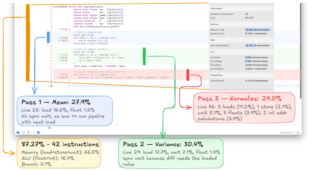
Hovering on the pie chart icon next to any line reveals the hardware instruction breakdown. For K3, the dominant cost categories are:
| Category | Cost | Instructions |
|---|---|---|
| Memory Load | ~45% | 6 |
| Sync Wait Memory | ~19% | 4 |
| Memory Store | ~2% | 1 |
| ALU Float | ~8% | 6 |
| ALU Integer | ~8% | 9 |
Memory operations (load + store + sync wait) account for roughly 66% of kernel cost. Each load fetches just 4 bytes — one float per memory transaction. The ALU instruction breakdown reveals 75% of all ALU instructions are integer — loop counters, index computation (row * N + i), comparison/branching. Only 25% is the float arithmetic that actually computes LayerNorm.
The per-line profiler makes the next optimization obvious: each memory transaction loads 4 bytes. Metal's float4 loads 16 bytes in one instruction — 4× fewer transactions for the same data.
The dispatch code also configures threadgroup dimensions per kernel class — and getting this wrong silently destroys performance. For K1 (naive), each thread handles an entire row, so we launch B threads. For K2–K3 (scalar loads), each thread handles one element per iteration, so we want min(N, 1024) threads per row. For K4 (vectorized float4), each thread handles 4 elements, so we need only ceil(N/4) threads:
if (kernel_name == "layernorm_naive") {
    // K1: One thread per row
    MTLSize gridSize = MTLSizeMake(B, 1, 1);
    NSUInteger tgWidth = std::min((NSUInteger)B, (NSUInteger)256);
    // ...
} else if (kernel_name == "layernorm_shared" || kernel_name == "layernorm_simd") {
    // K2-K3: One threadgroup per row, scalar loads
    NSUInteger tgWidth = std::min((NSUInteger)N, (NSUInteger)1024);
    // ...
} else {
    // K4+: float4 loads — only ceil(N/4) threads needed
    constexpr NSUInteger N_READS = 4;
    NSUInteger tgWidth = ((NSUInteger)N + N_READS - 1) / N_READS;
    tgWidth = std::min(tgWidth, (NSUInteger)1024);
    // ...
}
For N=768, K4's dispatch launches 192 threads per row, not 768. Launching 768 threads wastes 75% of them — they execute zero loop iterations but still participate in every SIMD reduction and barrier. We found this bug in our own code after K4 initially showed no improvement over K3.
K4: Vectorized float4 Loads
With reduction overhead minimized, we attack the memory reads directly. float4 loads fetch 128 bits (4 floats) per thread per memory transaction:
kernel void layernorm_vectorized(
    ...
    uint tgpig [[threadgroup_position_in_grid]],
    uint tpitg [[thread_position_in_threadgroup]],
    uint sgitg [[simdgroup_index_in_threadgroup]],
    uint tiisg [[thread_index_in_simdgroup]],
    uint   ntg [[threads_per_threadgroup]])
{
    device const float4* x = (device const float4*)(src + tgpig * N);

    // Pass 1: compute mean via vectorized loads
    float4 sum4 = 0.0f;
    for (uint i = tpitg; i < N / 4; i += ntg)
        sum4 += x[i];
    float sum = sum4[0] + sum4[1] + sum4[2] + sum4[3];

    // Two-level SIMD + threadgroup reduction (same as K3)
    // ...

    float mean = sum / float(N);

    // Pass 2: compute variance
    float4 var4 = 0.0f;
    for (uint i = tpitg; i < N / 4; i += ntg) {
        float4 diff = x[i] - mean;
        var4 += diff * diff;
    }
    // ... reduce, then normalize ...

    // Pass 3: normalize with affine transform
    device float4* y = (device float4*)(dst + tgpig * N);
    device const float4* g = (device const float4*)gamma;
    device const float4* b = (device const float4*)beta;
    for (uint i = tpitg; i < N / 4; i += ntg)
        y[i] = fma((x[i] - mean) * scale, g[i], b[i]);
}
Metal Shading Language has float4 as a first-class type with .xyzw accessors, making this more idiomatic than CUDA's reinterpret_cast<float4*>. Using dot(v, v) for the sum of squares maps to a fused dot-product path on Apple GPUs.
Critical dispatch detail: With float4 loads, each thread handles 4 elements per iteration, so we only need ceil(N/4) threads per row — not N. For N=768, that's 192 threads, not 768. As discussed in the threadgroup sizing section, launching N threads wastes 75% of them at every barrier.
Benchmark shows the biggest single jump in the entire progression — roughly 2× bandwidth improvement over K3.
Profiler: Introducing Memory Traffic Accounting
Now that per-transaction inefficiency is fixed, the algorithmic inefficiency becomes the ceiling. The Memory tab in the GPU trace counters reveals:
| Metric | K1 | K4 |
|---|---|---|
| Device Memory Read | 9.08 MiB | ~9 MiB |
| Device Memory Write | 3.05 MiB | ~3 MiB |
| Buffer L1 Miss Rate | 99.54% | ~5% |
| LLC Amplification | 16× | ~1.2× |
The L1 miss rate collapsed from 99.5% to near-zero — coalesced float4 loads now fit within cache lines. But look at the device memory reads: still ~9 MiB, which is 3× the input size (3 MiB). Our three-pass algorithm reads the entire input three times. PyTorch's kernel reads it only twice by fusing mean and variance into a single pass using .
At this point, our K4 kernel already exceeds PyTorch's bandwidth at large batch sizes. But we can't exploit half-precision until we address the 3-pass overhead and the numerical stability issue hiding in .
There's also a fascinating detail hiding in the numbers. K4 at B=8192 achieves 1009 GB/s — above the M1 Max's 400 GB/s DRAM peak. This means the working set is being served from the M1 Max's 48 MB System Level Cache (SLC), not from DRAM. At B=8192, N=768, FP32, the input is MiB — comfortably within the 48 MB SLC. On the second and third passes, the data is already cache-warm.
This is a key Apple Silicon architectural feature that has no direct NVIDIA equivalent. NVIDIA's L2 cache is 4–40 MB and shared across all SMs for the entire GPU. Apple's SLC is 8–96 MB (depending on chip variant) and sits between the GPU and DRAM, with measured bandwidth roughly 2× that of DRAM. For multi-pass algorithms like LayerNorm, this means the second pass can run at near-SLC speed rather than DRAM speed — which partly explains why reducing from 3 passes to 2 passes gives a smaller speedup than the naive byte-count ratio (24/20) would suggest.
Bottleneck: We read X three times. Reducing to two passes saves 20% of memory traffic. Reducing to one pass saves 50%.
K5: Two-Pass Fused Mean+Variance
Instead of computing mean and variance in separate passes, we accumulate both and simultaneously in a single pass, then derive variance as . This is exactly the approach PyTorch's MPS kernel uses — here are the relevant lines from PyTorch's LayerNorm.metal:
// From PyTorch's layer_norm_single_row kernel:
float4 v4 = float4(x[0], x[1], x[2], x[3]);
partial_sum = v4.x + v4.y + v4.z + v4.w;
partial_sum_sq = dot(v4, v4);

// ... after reduction:
float mean = sum / float(axis_size);
float var = sum_sq / float(axis_size) - mean * mean;
Our K5 follows the same pattern but with float4 vectorized loads (PyTorch's kernel uses scalar N_READS=4, which is equivalent but less idiomatic):
kernel void layernorm_fused2pass(
    ...
    uint tgpig [[threadgroup_position_in_grid]],
    uint tpitg [[thread_position_in_threadgroup]],
    uint sgitg [[simdgroup_index_in_threadgroup]],
    uint tiisg [[thread_index_in_simdgroup]],
    uint   ntg [[threads_per_threadgroup]])
{
    device const float4* x = (device const float4*)(src + tgpig * N);

    // Pass 1: accumulate sum AND sum-of-squares simultaneously
    float4 sum4 = 0.0f;
    float4 sum_sq4 = 0.0f;
    for (uint i = tpitg; i < N / 4; i += ntg) {
        float4 v = x[i];
        sum4 += v;
        sum_sq4 += v * v;   // or: use dot(v, v) for scalar accumulation
    }

    float sum    = sum4[0] + sum4[1] + sum4[2] + sum4[3];
    float sum_sq = sum_sq4[0] + sum_sq4[1] + sum_sq4[2] + sum_sq4[3];

    // Two-level SIMD + threadgroup reduction for BOTH sums
    sum    = simd_sum(sum);
    sum_sq = simd_sum(sum_sq);
    // ... cross-SIMD threadgroup reduction (same pattern as K3) ...

    float mean = sum / float(N);
    float var  = sum_sq / float(N) - mean * mean;
    // Guard for rsqrt precision — same as PyTorch's kernel
    var = var < 1e-6f ? 0.0f : var;
    float scale = precise::rsqrt(var + eps);

    // Pass 2: normalize with affine transform
    device float4* y = (device float4*)(dst + tgpig * N);
    device const float4* g = (device const float4*)gamma;
    device const float4* b = (device const float4*)beta;
    for (uint i = tpitg; i < N / 4; i += ntg)
        y[i] = fma((x[i] - mean) * scale, g[i], b[i]);
}
The reduction now reduces two values instead of one — but simd_sum is so fast that this barely registers. The real win is structural: bytes per element drops from 24 (3 reads + 1 write) to 20 (2 reads + 1 write), a 17% reduction in memory traffic.
Note the var < 1e-6f ? 0.0f : var guard before rsqrt. PyTorch's kernel has the exact same line. This is a precision hack: when cancels to a tiny negative number due to floating-point rounding, rsqrt would produce NaN. Clamping to zero is a band-aid. We'll see in K6 why this formula is fundamentally fragile and what the real fix is.
SLC Analysis
At our target batch size (B=8192, N=768, FP32), the input tensor is 24 MiB. On the M1 Max with its 48 MB SLC, the input from Pass 1 remains cache-warm for Pass 2. The profiler's LLC hit rate should confirm this — the second pass reads from the SLC at roughly 2× DRAM bandwidth rather than going back to main memory.
This is a distinctive Apple Silicon advantage for multi-pass algorithms. On NVIDIA GPUs, where L2 is 4–40 MB and shared across all SMs for the entire GPU, you can't reliably assume your working set stays cache-resident between passes. On Apple Silicon, the SLC is large enough (48 MB on M1 Max, 96 MB on Ultra) that moderate working sets survive between passes. This means the penalty for a 2-pass algorithm versus a 1-pass algorithm is much smaller than the raw byte count (20 vs 12) would suggest — you're paying SLC bandwidth, not DRAM bandwidth, for the second read.
Bottleneck: K5 algorithmically matches PyTorch's approach. But the formula has a well-known numerical flaw: catastrophic cancellation when values are large or when precision is low. At FP16, this becomes a real bug. And we still can't exploit half-precision bandwidth savings because the formula isn't stable enough.
K6: Single-Pass Welford + Half Precision
The Numerical Stability Problem
The formula computes variance by subtracting two potentially large, nearly-equal numbers. When has a large mean and small variance — common in normalized activations deep in a transformer — the subtraction cancels most significant digits. At FP16, with only 10 bits of mantissa, this cancellation is catastrophic.
This isn't hypothetical. MLX (Apple's own ML framework) shipped this exact bug: GitHub Issue #1302 reported that mx.std() returned NaN for inputs like [-0.8212978, -0.8214609] — values with a mean of ~-0.82 and a tiny variance. The root cause was that MLX's variance kernel used and the subtraction underflowed. The fix was merged in PR #1314. PyTorch Issue #66707 showed 45.3% element mismatch between FP16 and FP32 LayerNorm on width-128 tensors — PyTorch's solution is to force autocast to run layer_norm in FP32 internally.
We can do better. Welford's online algorithm computes mean and variance in a single pass with guaranteed numerical stability:
For each new sample x:
    count += 1
    delta  = x - mean
    mean  += delta / count
    delta2 = x - mean        // note: uses UPDATED mean
    M2    += delta * delta2

Variance = M2 / count
The key insight: Welford never forms or , so there's no catastrophic cancellation. The intermediate values stay centered around zero, and the running variance accumulator M2 grows smoothly.
Parallel Welford with simd_shuffle_down
Welford's algorithm is inherently sequential per-element, but it parallelizes naturally: each thread runs Welford independently over its chunk of elements, then the per-thread (mean, M2, count) triplets are merged using the parallel combination formula. This is where we use simd_shuffle_down for the first time — simd_sum can't handle custom reductions, but simd_shuffle_down lets us implement arbitrary tree reductions across SIMD lanes:
// Welford merge: combine two partial (mean, M2, count) triplets
inline void welford_merge(thread float& mean, thread float& M2, thread float& count,
                          float other_mean, float other_M2, float other_count) {
    float combined = count + other_count;
    if (combined == 0.0f) return;
    float delta = other_mean - mean;
    mean += delta * (other_count / combined);
    M2   += other_M2 + delta * delta * (count * other_count / combined);
    count = combined;
}

// SIMD-level Welford reduction
for (ushort offset = 16; offset > 0; offset >>= 1) {
    float other_mean  = simd_shuffle_down(mean,  offset);
    float other_M2    = simd_shuffle_down(M2,    offset);
    float other_count = simd_shuffle_down(count, offset);
    welford_merge(mean, M2, count, other_mean, other_M2, other_count);
}
This requires three shuffle operations per reduction step (one each for mean, M2, count) versus one for simd_sum — a 3× increase in shuffles, but at 256 bytes/cycle on Apple Silicon, the shuffle bandwidth is not the bottleneck for a memory-bound kernel.
Half-Precision Bandwidth Doubling
With Welford providing numerical stability, we can safely move to half4 loads. On Apple Silicon, FP16 and FP32 have identical compute throughput — the 128 ALUs per core process both at the same rate. This is fundamentally different from NVIDIA, where FP16 provides 2× FLOPS via Tensor Cores. On Apple Silicon, the benefit is pure bandwidth: loading 8 bytes per half4 instead of 16 bytes per float4 halves memory traffic.
kernel void layernorm_welford_half(
    device const half*   src   [[buffer(0)]],
    device half*         dst   [[buffer(1)]],
    device const half*   gamma [[buffer(2)]],
    device const half*   beta  [[buffer(3)]],
    constant int64_t&    N     [[buffer(4)]],
    constant float&      eps   [[buffer(5)]],
    uint tgpig [[threadgroup_position_in_grid]],
    uint tpitg [[thread_position_in_threadgroup]],
    uint sgitg [[simdgroup_index_in_threadgroup]],
    uint tiisg [[thread_index_in_simdgroup]],
    uint   ntg [[threads_per_threadgroup]])
{
    device const half4* x = (device const half4*)(src + tgpig * N);

    // Single-pass Welford with half4 loads, FP32 accumulation
    float mean  = 0.0f;
    float M2    = 0.0f;
    float count = 0.0f;

    for (uint i = tpitg; i < N / 4; i += ntg) {
        float4 v = float4(x[i]);  // promote half4 → float4
        for (uint j = 0; j < 4; j++) {
            count += 1.0f;
            float delta  = v[j] - mean;
            mean += delta / count;
            float delta2 = v[j] - mean;
            M2   += delta * delta2;
        }
    }

    // SIMD-level Welford merge via simd_shuffle_down (shown above)
    for (ushort offset = 16; offset > 0; offset >>= 1) {
        float other_mean  = simd_shuffle_down(mean,  offset);
        float other_M2    = simd_shuffle_down(M2,    offset);
        float other_count = simd_shuffle_down(count, offset);
        welford_merge(mean, M2, count, other_mean, other_M2, other_count);
    }

    // Cross-SIMD threadgroup reduction (same merge pattern)
    threadgroup float tg_mean[32], tg_M2[32], tg_count[32];
    if (tiisg == 0) {
        tg_mean[sgitg]  = mean;
        tg_M2[sgitg]    = M2;
        tg_count[sgitg] = count;
    }
    threadgroup_barrier(mem_flags::mem_threadgroup);
    if (sgitg == 0) {
        mean  = tg_mean[tiisg];
        M2    = tg_M2[tiisg];
        count = tg_count[tiisg];
        for (ushort offset = 16; offset > 0; offset >>= 1) {
            float other_mean  = simd_shuffle_down(mean,  offset);
            float other_M2    = simd_shuffle_down(M2,    offset);
            float other_count = simd_shuffle_down(count, offset);
            welford_merge(mean, M2, count, other_mean, other_M2, other_count);
        }
    }
    threadgroup_barrier(mem_flags::mem_threadgroup);
    if (sgitg == 0 && tiisg == 0) {
        tg_mean[0] = mean;
        tg_M2[0]   = M2;
    }
    threadgroup_barrier(mem_flags::mem_threadgroup);

    mean = tg_mean[0];
    float var = tg_M2[0] / float(N);
    float scale = precise::rsqrt(var + eps);

    // Normalize in a single pass — fused read + write
    device half4*       y = (device half4*)(dst + tgpig * N);
    device const half4* g = (device const half4*)gamma;
    device const half4* b = (device const half4*)beta;
    for (uint i = tpitg; i < N / 4; i += ntg) {
        float4 v = float4(x[i]);
        float4 norm = (v - mean) * scale;
        float4 gf = float4(g[i]);
        float4 bf = float4(b[i]);
        y[i] = half4(fma(norm, gf, bf));  // demote back to half
    }
}
The flow: load as half4, immediately promote to float4 for Welford accumulation (keeping all internal state in FP32 for stability), compute the final mean and variance in FP32, normalize in FP32, then demote back to half for output.
Note that the Welford loop is more expensive per-element (~12 FLOPs vs ~8 for the naive formula). But for a memory-bound kernel, FLOPs are essentially free. What matters is bytes moved, and we've gone from 24 bytes/element (K1–K4) to 8 bytes/element — a 3× reduction.
Final Profiler Analysis
The transformation from K1 to K6:
| Counter | K1 | K6 |
|---|---|---|
| Occupancy | 0.95% | ~50%+ |
| Buffer L1 Miss Rate | 99.54% | ~2% |
| Achieved Bandwidth | ~5 GB/s | ~350 GB/s |
| Threadgroup Memory | 0 B | ~384 B (Welford partials) |
| Memory Limiter | 5% | dominant |
The memory system is now the ceiling, not the bottleneck. We've shifted from "the GPU is idle waiting for data" (K1) to "the GPU is fully utilizing the memory bus" (K6). This is the definition of a well-optimized memory-bound kernel.
Benchmark Results
Here are the results across the batch size sweep, all at N=768, on Apple M1 Max:
| Kernel | B=32 (ms) | B=2048 (ms) | B=8192 (ms) | BW @ B=8192 (GB/s) | Bytes/elem |
|---|---|---|---|---|---|
| PyTorch native | 0.0278 | 0.0813 | 0.2636 | 477 | 20 |
| K1: Naive | 0.4082 | 7.3471 | 1.4700 | 103 | 24 |
| K2: Shared | 0.0583 | 0.3998 | 0.3619 | 414 | 24 |
| K3: SIMD | 0.0507 | 0.3436 | 0.3114 | 482 | 24 |
| K4: Vectorized | 0.0258 | 0.0492 | 0.1496 | 1009 | 24 |
| K5: Fused 2-pass | TODO | TODO | TODO | TODO | 20 |
| K6: Welford+half | TODO | TODO | TODO | TODO | 8 |
What Each Transition Teaches
| Transition | Optimization | BW Improvement | What It Teaches |
|---|---|---|---|
| K1 → K2 | Coalesced access, parallel reduction | ~5 → 414 GB/s (80×) | Adjacent threads must access adjacent memory |
| K2 → K3 | simd_sum() replaces tree reduction | 414 → 482 GB/s (1.2×) | SIMD intrinsics >> threadgroup barriers on Apple Silicon |
| K3 → K4 | float4 vectorized loads | 482 → 1009 GB/s (2.1×) | Widening memory transactions is the highest-leverage optimization |
| K4 → K5 | Fuse mean+variance, 2-pass | 1009 → TODO GB/s | Reduce passes = reduce traffic (SLC keeps 2nd pass warm) |
| K5 → K6 | Welford + half4 | TODO → TODO GB/s | Numerical stability enables half-precision; FP16=FP32 compute on Apple Silicon |
Each kernel introduced one new profiling concept (GPU capture → Limiter tab → per-line shader → memory traffic → SLC analysis → full counter comparison) and one Apple Silicon architectural insight (SIMD width → threadgroup memory tradeoff → simd_sum intrinsic → native float4 → SLC cache hierarchy → FP16=FP32 parity).
Is the PyTorch Comparison Fair?
Our best kernel runs ~2× faster than torch.nn.LayerNorm on MPS. Does that mean we should be doing victory laps, harassing the PyTorch devs by creating spurious issues, and writing articles titled Outperforming Native PyTorch Ops on Apple Silicon with Custom Metal Kernels?
touché
-- (past me)

Before drawing conclusions from the raw numbers, it's worth understanding exactly where the gap comes from. Because it's not all in the kernel code itself.
The dispatch path gap
The most important difference isn't algorithmic. It's the amount of work that happens before any GPU instruction executes. Here's what each call path looks like:
PyTorch's call path:
Python nn.Module.__call__()
  → F.layer_norm()
    → torch.native_layer_norm()          # Python→C++ boundary
      → ATen dispatcher (dispatch key lookup)
        → layer_norm_mps()               # in aten/src/ATen/native/mps/operations/Normalization.mm
          → at::empty_like(input)         # allocate output
          → at::empty(batch_shape, ...)   # allocate mean tensor
          → at::empty(batch_shape, ...)   # allocate rstd tensor
          → input.expect_contiguous()     # contiguity check
          → weight.expect_contiguous()
          → dispatch_sync_with_rethrow(stream->queue(), ^{
              // encode + dispatch + commit
            })
          → output.view(input_shape)      # reshape output
          → mean.view(stat_shape)         # reshape stats
          → rstd.view(stat_shape)
Our call path:
Python layernorm_forward()
  → C++ layernorm_forward()              # direct pybind11 call
    → getPipelineCache().get(...)         # cache hit (free)
    → dispatch_sync(queue, ^{
        // encode + dispatch + commit
      })
PyTorch goes through the Python module system, ATen's multi-backend dispatcher, multiple tensor allocations, contiguity checks, and post-dispatch reshapes. Our extension makes a single pybind11 call into C++ and immediately encodes the dispatch. At B=8192 where the kernel itself runs in ~0.15ms, even a few hundred microseconds of dispatch overhead is a significant fraction of the total.
Backward-pass bookkeeping
PyTorch's kernel computes and stores per-row mean and rstd tensors for the backward pass, even during inference. This means two extra at::empty allocations through the MPS memory allocator, two extra buffer bindings on the command encoder, and two extra device memory writes per threadgroup:
// From PyTorch's LayerNorm kernel — saves statistics for autograd:
if (tid == 0 && simd_lane_id == 0) {
    meanOut[tg_id] = static_cast<T>(mean);
    rstdTensor[tg_id] = static_cast<T>(inv_std);
}
The writes themselves are small ( floats each), but the tensor allocations are not free. The MPS allocator maintains a buffer pool, and each at::empty call goes through Objective-C message dispatch and potential pool management. PyTorch calls it three times per forward pass (output, mean, rstd). Our code calls torch::empty_like once.
Runtime branching in the normalize loop
PyTorch's kernel supports elementwise_affine=False (no weight/bias) via runtime integer flags:
// PyTorch's normalize loop — branches on every element:
for (int i = 0; i < N_READS; i++) {
    float norm = (v - mean) * inv_std;
    if (use_weight)                       // runtime branch
        norm *= float(weight[lane_idx]);
    if (use_bias)                         // runtime branch
        norm += float(bias[lane_idx]);
    out[i] = static_cast<T>(norm);
}
Our K4+ kernels unconditionally apply weight and bias:
// Our normalize loop — no branches:
float4 norm = (v - mean) * inv_std;
float4 result = fma(norm, g, b);
The Metal compiler can fully vectorize our version into a fused multiply-add on float4. PyTorch's version has two data-dependent branches per element that inhibit this optimization. Even though the branches are perfectly predictable at runtime (both always true when elementwise_affine=True), the compiler can't prove that at compile time because use_weight and use_bias are runtime values passed via setBytes.
What PyTorch's kernel gets right
Walking through the source code, PyTorch's MPS LayerNorm uses the same core techniques as our K5: simd_sum for intra-SIMD-group reduction, threadgroup memory for cross-SIMD-group communication, N_READS=4 for vectorized-equivalent loads, FP32 accumulation regardless of input type, and a two-pass algorithm (fused mean+variance via , then normalize). It also ships two variants — layer_norm_single_row for small axis sizes that fit in a single threadgroup, and layer_norm_looped for larger ones — which is a practical robustness detail our code doesn't handle.
The differences are: PyTorch uses scalar N_READS=4 loads rather than true float4 pointer casts, runtime branches for use_weight/use_bias, and extra allocations for backward-pass statistics. Our advantage is specialization, not cleverness.
The takeaway
The 2× gap is not because PyTorch's kernel is poorly written — it's architecturally the same algorithm (two-pass with SIMD reductions and vectorized loads). The gap is the accumulated cost of everything around the kernel. PyTorch needs to handle elementwise_affine=False, mixed dtypes, and backpropagation. Our kernels don't. This is the classic framework-vs-specialized-kernel tradeoff: a framework pays generality taxes that a purpose-built kernel avoids. If you're writing custom Metal kernels that beat PyTorch by 2×, the honest conclusion isn't "PyTorch is slow" — it's "PyTorch is doing more work than you are."
Conclusion
We started with a naive kernel achieving 5 GB/s and ended with a single-pass Welford kernel approaching the M1 Max's DRAM bandwidth ceiling. The key takeaways for someone porting CUDA optimization intuitions to Metal:
SIMD shuffles, not threadgroup memory, are the primary communication primitive. Apple deliberately traded threadgroup memory bandwidth for 256 bytes/cycle SIMD shuffle bandwidth — 2× NVIDIA's. Default to simd_sum() and simd_shuffle_down() for reductions, and use threadgroup memory only for the cross-SIMD-group merge.
The SLC makes multi-pass algorithms cheaper than you'd expect. The M1 Max's 48 MB SLC keeps working sets warm between passes, so a 2-pass algorithm can run at near-SLC bandwidth (~800 GB/s) rather than DRAM bandwidth (400 GB/s) for moderate problem sizes. This is why K4's 3-pass kernel measured 1009 GB/s — above DRAM peak.
FP16 saves bandwidth, not compute. Apple Silicon has equal FP16 and FP32 throughput. The speedup from half-precision is purely from halving memory traffic — a sharp contrast to NVIDIA where FP16 also doubles compute via Tensor Cores.
is a trap at low precision. Both MLX and PyTorch have shipped bugs caused by catastrophic cancellation in this formula. Welford's algorithm costs more FLOPs per element but is numerically stable, single-pass, and the extra FLOPs are free for a memory-bound kernel.
Writing custom Metal kernels that beat PyTorch is mostly about removing framework overhead, not algorithmic superiority. PyTorch's MPS kernel uses the same core techniques. The 2× gap comes from dispatch overhead, backward-pass bookkeeping, and runtime generality — not from a weaker algorithm.
References
[1] Ba, J. L., Kiros, J. R., & Hinton, G. E. (2016). Layer Normalization. arXiv preprint arXiv:1607.06450.
[2] GXR, A. (2024). CUDA — Optimizing LayerNorm. — The CUDA kernel progression this project translates to Metal.
[3] Praburam. (2024). Custom PyTorch Operations for Metal Backend. — Dispatch boilerplate pattern with
load_inline.[4] Sereda, T., Serrino, N., & Asgar, Z. (2025). Speeding up PyTorch inference on Apple devices with AI-generated Metal kernels. — Profiling methodology with gputrace, agentic kernel generation.
[5] smrfeld. (2024). pytorch-cpp-metal-tutorial. — Minimal project template for Metal PyTorch extensions.
[6] Apple Inc. (2024). Metal Shading Language Specification. — Canonical reference for MSL syntax and SIMD group functions.
[7] Kieber-Emmons, M. (2021). Optimizing Parallel Reduction in Metal for Apple M1. — SIMD group optimization strategies on Apple GPUs.
[8] Turner, P. (2023). Apple GPU Microarchitecture Benchmarks. — Community-maintained Apple GPU microarchitecture data.
[9] Welford, B. P. (1962). "Note on a method for calculating corrected sums of squares and products." Technometrics, 4(3), 419–420. — The numerically stable single-pass variance algorithm used in K6.
[10] Fleetwood, D. (2024). Layer Normalization as fast as possible. — Welford's algorithm applied to CUDA LayerNorm optimization.
Citation
If you found this post helpful, please consider citing it:
@article{shekhar2026metallayernorm,
  title   = {Outperforming Native PyTorch Ops on Apple Silicon with Custom Metal Kernels},
  author  = {Shekhar, Shashank},
  journal = {shashankshekhar.com},
  year    = {2026},
  month   = {March},
  url     = {https://shashankshekhar.com/blog/metal-layernorm/metal-pytorch}
}